All of MFCC

Sound is a wave. To store sound in a computer, waves of air pressure are converted into voltage via a microphone and sampled with an analog-to-digital converter where the output is stored as a one-dimensional array of numbers. Simply saying, an audio file is just an array of amplitudes sampled with a certain rate known as the sampling rate and it has a sample rate, number of channels of sound, and precision (bit depth) as meta-property.

Standard telephone audio has a sampling rate of 8 kHz and 16-bit precision.

You might have heard a familiar term called bit-rate (bit per second), which measures the overall quality of audio.

bitrate = sample rate x precision x no. of channels

A raw audio signal is high-dimensional and difficult to model as there is much information and it consists of many unwanted signals, especially in the case of human speech sound.

Mel-frequency Cepstrum Coefficients (MFCC) tries to model the audio in a format where it performs those type of filtering that correlates to the human auditory system and their low dimensionality. It is the most commonly used feature in Automatic Speech Recognition (ASR). Mel-frequency Cepstrum (MFC) is a representation of the short-term power spectrum of a sound, based on a linear cosine transform of a log power spectrum on a non-linear Mel-scale of frequency and MFCC are the coefficients that collectively make up the MFC.

Following are the steps to compute MFCC.

I will use an example sound wave and process it in python to make it more clear.

import librosa 
import numpy as np 
import librosa.display
import matplotlib.pyplot as plt
import sounddevice as sd
y, sr = librosa.load("00a80b4c8a.flac", sr=16000)

Pre-emphasis

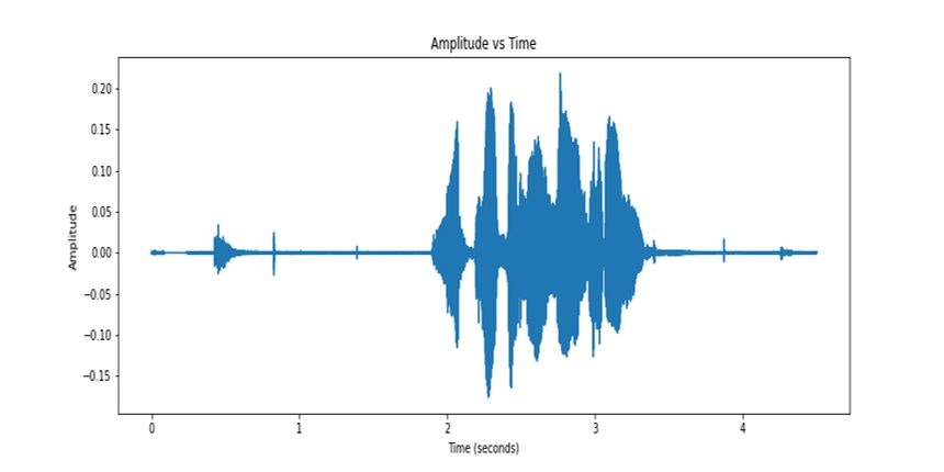
This is the first step in feature generation. In speech production, high frequencies usually have smaller magnitudes compared to lower frequencies. So in order to counter the effect, we apply a pre-emphasis signal to amply the amplitude of high frequencies and lower the amplitude of lower frequencies.

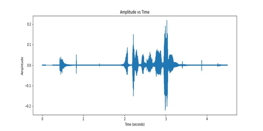
alpha = 0.97
y_emp = np.append(y[0], y[1:] - alpha * y[:-1])

Here's the visualization of the pre-emphasized signal.

Framing

An acoustic signal is perpetually changing in speech. But studies show that the characteristics of voice signals remain fixed in a short interval of time (called quasi-stationary signals). So while modeling the signal we take a small segment from the audio for further processing.

Separating the samples into fixed-length segments is known as framing or frame blocking. These frames are usually from 5 milliseconds to 100 milliseconds. But in the case of a speech signal, to preserve the phonemes, we often take the length of 20-40 milliseconds, which is usually the length of phonemes with 10-15 milliseconds overlap.

These segments are later converted to the frequency domain with an FFT.

Why do we use overlapping of the frames?

We can imagine a non-overlapping rectangular frame. Each sample is, somehow, treated with the same weight. However, when we process the features extracted from two consecutive frames, the change of property between the frames may induce a discontinuity, or a jump ("the difference of parameter values of neighboring frames can be higher"). This blocking effect can create disturbance in the signal.

In Python, the array of amplitude is framed as:

frame_size = 0.02
frame_stride = 0.01 # frame overlap = 0.02 - 0.01 = 0.01 (10ms)

frame_length, frame_step = int(round(frame_size * sr)), int(round(frame_stride * sr))  # Convert from seconds to samples
signal_length = len(yemp)

num_frames = int(np.ceil(float(signal_length - frame_length) / frame_step))  # Make sure that we have at least 1 frame

pad_signal_length = num_frames * frame_step + frame_length
z = np.zeros((pad_signal_length - signal_length))
# Pad Signal to make sure that all frames have equal number of samples without truncating any samples from the original signal
pad_signal = np.append(yemp, z) 

indices = np.tile(np.arange(0, frame_length), (num_frames, 1)) + np.tile(np.arange(0, num_frames * frame_step, frame_step), (frame_length, 1)).T
frames = pad_signal[indices.astype(np.int32, copy=False)]

Windowing

Windowing multiplies the samples by a scaling function. This is done to eliminate discontinuities at the edges of the frames. If the function of windows is defined as w(n), 0 < n < N-1 where N is the number of samples per frame, the resulting signal will be;

Generally, hamming windows are used where

Why do we use windowing?

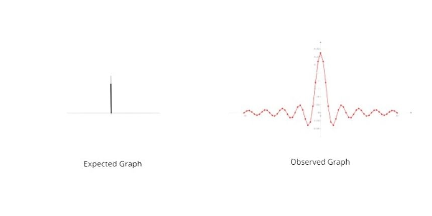
When we are changing signals from the time domain using FFT, we cannot perform computations on infinite data points with computers so all signals are cut off at either end. For example, let's say we want to do FFT on a pure sine wave. In the frequency domain, we expect a sharp spike in the respective frequency of the sine wave. But when we visualize it, we see a ripple-like graph on many frequencies which is not even the frequency of the wave.

When we cut off the signal at either end, we are indirectly multiplying our signal by a square window. So there is a variety of window functions people have come up with. Hamming window, analytically, is known to optimize the characteristics needed for speech processing.

Fourier Transform 

Fourier transform (FT) is a mathematical transform that decomposes a function (often a function of time, or a signal) into its constituent frequencies. This is used to analyze frequencies contained in the speech signal. And it also gives the magnitude of each frequency.

where, k = 0, 1, 2, ... , N-1

Short-time Fourier transform (STFT) converts the 1-dimensional signal from the time domain into the frequency domain by using the frames and applying a discrete Fourier transform to each frame. We can now do an N-point FFT on each frame to calculate the frequency spectrum, which is also called Short-Time Fourier-Transform (STFT). STFT provides the time-localized frequency information because, in speech signals, frequency components vary over time. Usually, we take N=256.

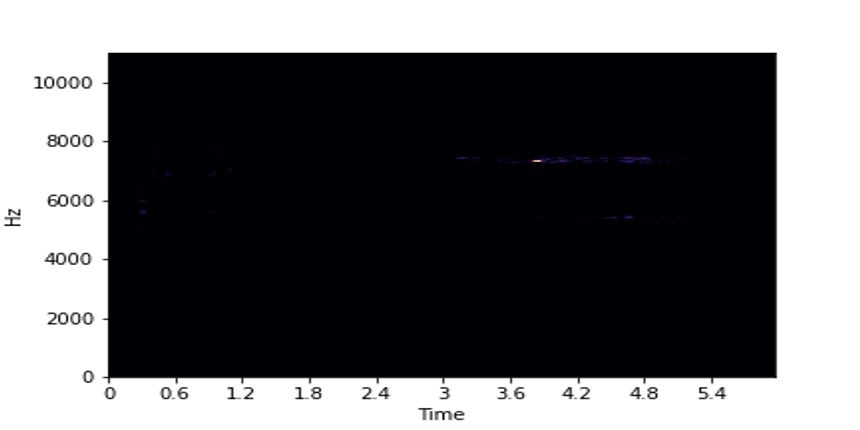
Spectrogram: A spectrogram is a visual representation of the spectrum of frequencies of a signal as it varies with time. For some end-to-end systems, spectrograms are taken as input. This helps in the 3D visualization of the FFT. The magnitude of Spectrogram Sm=|FFT(xi)|2 Power Spectrogram Sp=SmN Where N is the number of points considered for FFT computation. (typically 256 or 512)

In Python:

NFFT = 512
magnitude = np.absolute(np.fft.rfft(frames, NFFT))
pow_frames = magnitude**2/NFFT

Mel-Filter Bank

The magnitude spectrum is warped according to the Mel scale to adapt the frequency resolution to the non-linear properties of the human ear by being more discriminative at lower frequencies and less discriminative at higher frequencies. We can convert between Hz scale and Mel scale using the following equations:

The parameters that define a Mel filter bank are: